
Crea elenco in Excel: una guida rapida
Con il cambiamento dell'orario di lavoro, non è sempre facile avere una visione d'insieme. Un elenco semplice in Excel può essere molto utile. Ti mostriamo come creare rapidamente un turno o un piano di lavoro con Office 2010.
La struttura del piano di turni
Il nostro elenco è composto essenzialmente da soli tre componenti:
- L'intestazione, in cui sono elencati i diversi tipi di turno e i tempi associati.
- La barra laterale con la data e il giorno della settimana
- La tabella in cui inserisci i tuoi rispettivi livelli.

Piano di turni per i lavoratori
Questo elenco è destinato principalmente ai lavoratori che desiderano scrivere i propri turni.
- Se desideri creare un elenco per i tuoi dipendenti, segui prima queste istruzioni.
- Quindi aggiungi semplicemente alcune righe nei giorni della settimana, a seconda di quanti dipendenti lavorano per turno.
- Qui inserisci i nomi dei tuoi dipendenti che desideri assegnare ai turni pertinenti.
1. Il formato del calendario di lavoro
Innanzitutto, formatta le righe e le colonne in base alle tue esigenze.
- Vai all'intestazione della colonna e fai clic sulla colonna D.
- Spostare il mouse sul limite della linea destra e trascinare la colonna su una larghezza di 5 cm.
- Fare doppio clic sul "simbolo del formato" nella barra di avvio rapido del "menu Start".
- Quindi formatta le colonne F, H, J e L di 5 cm di larghezza allo stesso modo.
- Aumenta le colonne E, G, I e K a 15 cm ciascuna.
- Per la colonna M, selezionare una larghezza di 30 cm.

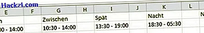
2. Etichettare l'intestazione del roster
Inserisci i tipi di turno nell'intestazione. Nel nostro esempio, si tratterebbe dei turni precoci, intermedi, tardivi e notturni. Se hai meno o più livelli, regola semplicemente i campi di conseguenza.
- Nella prima riga inizi con la cella A1 e inserisci "Gennaio" o un altro mese lì.
- Cella E1: presto
- Cella G1: tra
- Cella I1: in ritardo
- Cella K1: notte
- Cella M1: note
- Nella seconda riga, scrivi i rispettivi orari di ufficio.
3. Formattare le fasce orarie nel programma turni
Come spesso accade, ci sono ovviamente una vasta gamma di opzioni di design. Nel nostro esempio, abbiamo scelto due colonne, ognuna delle quali elenca la data e il giorno della settimana associato.
- Fai clic sulla colonna B nell'intestazione del foglio di lavoro.
- Fare clic con il tasto destro del mouse per aprire il menu di scelta rapida.
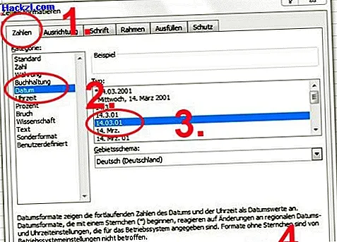
- Seleziona l'opzione "Formato celle".
- Quindi fai clic sulla scheda "Numeri".
- Nella "Categoria" selezionare "Data".
- Sotto "Tipo" selezionare la quinta voce nel modulo "14.03.01".
- Confermare la selezione con "OK".
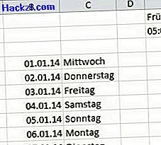
4. Riempi le due colonne del roster con la vita
Nel passaggio successivo inserisci rapidamente la data e il giorno della settimana.
- Nel primo passaggio, fai clic sulla cella B4.
- Inserisci qui la data "01/01/14".
- Quindi fai clic sul quadratino che vedi in basso a destra e tieni premuto il pulsante del mouse. Trascina il mouse verso il basso fino a quando viene visualizzato l'ultimo giorno del mese.
- La procedura nella cella C4 è quasi identica. Clicca sulla cella.
- Inserisci il primo giorno della settimana, nel nostro caso mercoledì.
- Quindi fai lo stesso della data. Fai clic sul quadratino nero e trascina i giorni della settimana verso il basso con il pulsante sinistro del mouse premuto fino alla fine del mese.
5. Tocchi finali sul tuo calendario di lavoro
Infine, alcune misure visive come la dimensione del carattere, il carattere in grassetto e il fissaggio della riga superiore. Grazie alla fissazione, puoi ancora vedere l'intestazione del piano di turni anche se devi scorrere verso il basso. Puoi trovare ulteriori suggerimenti sull'argomento "Caratteri in Excel" qui.
- Fare clic sul bordo della linea 1. Utilizzare i simboli nella parte superiore del programma per impostare la dimensione del carattere su 14 e in grassetto e centrare il testo.
- Nella riga 2, imposta la dimensione del carattere su 12 e allinea anche il testo al centro.
- Seleziona la scheda "Visualizza" nella parte superiore del programma.
- Fare clic sulla voce di menu "Congela finestra".
- Seleziona l'opzione "Congela linea superiore" dal menu contestuale.

Ora regoliamo i frame.
- Quindi segna le celle da E5 a K4 e fino a E34 - K34.
- Premi il pulsante destro del mouse e fai clic su "Formato celle" nel menu contestuale.
- Seleziona la scheda "Cornice".
- Seleziona il tipo "Interno" in "Preferenze".
- Confermare con "OK".
- Tenere premuto il tasto [CTRL] e fare clic sulle colonne F, H, J e L.
- Vai al simbolo della tabella nel menu a schede e seleziona "Nessun frame".

6. Immettere i servizi
Ora puoi inserire i tuoi livelli, ad esempio scrivendo in X nella cella corrispondente. Oppure puoi fare clic nella cella corrispondente e utilizzare il pulsante "Riempi celle" per selezionare un bel colore con cui contrassegnare il servizio.
- Nel nostro esempio, abbiamo anche evidenziato le domeniche a colori per maggiore chiarezza. Per fare ciò, segna le celle corrispondenti e seleziona un colore adatto con il pulsante "Riempi celle".
Se si desidera creare subito un calendario annuale, è sufficiente copiare il calendario dei servizi appena creato e modificare le due colonne, la data e il giorno della settimana. Qui puoi scoprire come rinominare i singoli fogli di lavoro nella scheda qui sotto.